1. echopype Tour#

https://github.com/OSOceanAcoustics/echopype-examples/blob/main/notebooks/

A quick tour of core echopype capabilities.

1.1. Introduction#

1.1.1. Goals#

Illustrate a common workflow for echosounder data conversion, calibration and use. This workflow leverages the standardization applied by echopype and the power, ease of use and familiarity of libraries in the scientific Python ecosystem.
Extract and visualize data with relative ease.

1.1.2. Description#

This notebook uses EK60 echosounder data collected during the 2017 Joint U.S.-Canada Integrated Ecosystem and Pacific Hake Acoustic Trawl Survey (‘Pacific Hake Survey’) to illustrate a common workflow for data conversion, calibration and analysis using echopype and core scientific Python software packages, particularly xarray, GeoPandas and pandas.

Two days of cloud-hosted .raw data files are accessed by echopype directly from an Amazon Web Services (AWS) S3 “bucket” maintained by the NOAA NCEI Water-Column Sonar Data Archive. With echopype, each file is converted to a standardized representation based on the SONAR-netCDF4 v1.0 convention and saved to the Zarr cloud-optimized file format.

Data stored in the Zarr (or netCDF) file format using the SONAR-netCDF4 convention can be conveniently and intuitively manipulated with xarray in combination with related scientific Python packages. Mean Volume Backscattering Strength (MVBS) is computed with echopype from the combined, converted raw data files, after calibration. The GPS location track and MVBS echograms are visualized.

1.1.3. Running the notebook#

This notebook can be run with a conda environment created using the conda environment file https://github.com/OSOceanAcoustics/echopype-examples/blob/main/binder/environment.yml. The notebook creates the ./exports directory, if not already present. Zarr files will be exported there.

import glob
from pathlib import Path

import fsspec
import geopandas as gpd
import xarray as xr

import matplotlib.pyplot as plt
import cartopy.crs as ccrs
import cartopy.io.img_tiles as cimgt
from cartopy.mpl.gridliner import LONGITUDE_FORMATTER, LATITUDE_FORMATTER
import hvplot.xarray

import echopype as ep

import warnings
warnings.simplefilter("ignore", category=DeprecationWarning)

1.2. Compile list of raw files to read from the NCEI WCSD S3 bucket#

We’ll compile a list of several EK60 .raw files from the 2017 Pacific Hake survey, available via open, anonymous access from an AWS S3 bucket managed by the NCEI WCSD.

After using fsspec to establish an S3 “file system” access point, extract a list of .raw files in the target directory.

fs = fsspec.filesystem('s3', anon=True)

bucket = "ncei-wcsd-archive"
rawdirpath = "data/raw/Bell_M._Shimada/SH1707/EK60"

s3rawfiles = fs.glob(f"{bucket}/{rawdirpath}/*.raw")

print(f"There are {len(s3rawfiles)} raw files in the directory")

There are 4343 raw files in the directory

# print out the last two S3 raw file paths in the list
s3rawfiles[-2:]

['ncei-wcsd-archive/data/raw/Bell_M._Shimada/SH1707/EK60/Summer2017-D20170913-T180733.raw',
 'ncei-wcsd-archive/data/raw/Bell_M._Shimada/SH1707/EK60/Winter2017-D20170615-T002629.raw']

Each of these .raw files is typically about 25 MB. To select a reasonably small but meaningful target for this demo, let’s select all files from 2017-07-28 collected over a two hour period, 18:00 to 19:59 UTC. This is done through string matching on the time stamps found in the file names.

s3rawfiles = [
    s3path for s3path in s3rawfiles 
    if any([f"D2017{dtstr}" in s3path for dtstr in ['0728-T18', '0728-T19']])
]

print(f"There are {len(s3rawfiles)} target raw files available")

There are 5 target raw files available

s3rawfiles

['ncei-wcsd-archive/data/raw/Bell_M._Shimada/SH1707/EK60/Summer2017-D20170728-T181619.raw',
 'ncei-wcsd-archive/data/raw/Bell_M._Shimada/SH1707/EK60/Summer2017-D20170728-T184131.raw',
 'ncei-wcsd-archive/data/raw/Bell_M._Shimada/SH1707/EK60/Summer2017-D20170728-T190728.raw',
 'ncei-wcsd-archive/data/raw/Bell_M._Shimada/SH1707/EK60/Summer2017-D20170728-T193459.raw',
 'ncei-wcsd-archive/data/raw/Bell_M._Shimada/SH1707/EK60/Summer2017-D20170728-T195219.raw']

1.3. Read target raw files directly from AWS S3 bucket and convert to netcdf#

Create the directory where the exported files will be saved, if this directory doesn’t already exist.

converted_dpath = Path('exports')
converted_dpath.mkdir(exist_ok=True)

EchoData is an echopype object for conveniently handling raw converted data from either raw instrument files or previously converted and standardized raw netCDF4 and Zarr files. It is essentially a container for multiple xarray.Dataset objects, each corresponds to one of the netCDF4 groups specified in the SONAR-netCDF4 convention – the convention followed by echopype. The EchoData object can be used to conveniently accesse and explore the echosounder raw data and for calibration and other processing.

For each raw file:

Access file directly from S3 via ep.open_raw to create a converted EchoData object in memory
Add global and platform attributes to EchoData object
Export to a local Zarr file

for s3rawfpath in s3rawfiles:
    raw_fpath = Path(s3rawfpath)
    try:
        # Access file directly from S3 to create a converted EchoData object in memory
        ed = ep.open_raw(
            f"s3://{s3rawfpath}",
            sonar_model='EK60',
            storage_options={'anon': True}
        )
        # Manually populate additional metadata about the dataset and the platform
        # -- SONAR-netCDF4 Top-level Group attributes
        ed['Top-level'].attrs['title'] = "2017 Pacific Hake Acoustic Trawl Survey"
        ed['Top-level'].attrs['summary'] = (
            f"EK60 raw file from the {ed['Top-level'].attrs['title']}, "
            "converted to a SONAR-netCDF4 file using echopype."
        )
        # -- SONAR-netCDF4 Platform Group attributes
        ed['Platform'].attrs['platform_type'] = "Research vessel"
        ed['Platform'].attrs['platform_name'] = "Bell M. Shimada"  # A NOAA ship
        ed['Platform'].attrs['platform_code_ICES'] = "315"        
        
        # Save to converted Zarr format 
        # Use the same base file name as the raw file but with a ".zarr" extension        
        ed.to_zarr(save_path=converted_dpath, overwrite=True)
    except Exception as e:
        print(f"Failed to process raw file {raw_fpath.name}: {e}")

Let’s examine the last EchoData object created above, ed. This summary shows a collapsed view of the netCDF4 groups that make up the EchoData object, where each group corresponds to an xarray Dataset. The backscatter data is in the Sonar/Beam_group1 group, accessible as ed['Sonar/Beam_group1'].

print(f"Number of ping times in this EchoData object: {len(ed['Sonar/Beam_group1'].ping_time)}")

Number of ping times in this EchoData object: 523

Assemble a list of EchoData objects from the converted Zarr files and combine them into a single EchoData object using the combine_echodata function. By default open_converted lazy loads individual Zarr files and only metadata are read into memory, until more operations are executed, which in this case is the combine_echodata function (note: combine_echodata first writes out a temporary Zarr file locally).

ed_list = []
for converted_file in sorted(glob.glob(str(converted_dpath / "*.zarr"))):
    ed_list.append(ep.open_converted(converted_file))

combined_ed = ep.combine_echodata(ed_list, overwrite=True)

print(f"Number of ping times in the combined EchoData object: {len(combined_ed['Sonar/Beam_group1'].ping_time)}")

Number of ping times in the combined EchoData object: 2379

The Provenance group now of the combined EchoData object contains some helpful information compiled from the source files.

combined_ed['Provenance']

<xarray.Dataset>
Dimensions:                     (echodata_filename: 5, environment_attr_key: 0,
                                 filenames: 5, platform_attr_key: 3,
                                 platform_nmea_attr_key: 1,
                                 provenance_attr_key: 4, sonar_attr_key: 6,
                                 sonar_beam_group1_attr_key: 2,
                                 top_level_attr_key: 9,
                                 vendor_specific_attr_key: 0)
Coordinates:
  * echodata_filename           (echodata_filename) <U33 'Summer2017-D2017072...
  * environment_attr_key        (environment_attr_key) float64 
  * filenames                   (filenames) int64 0 1 2 3 4
  * platform_attr_key           (platform_attr_key) <U18 'platform_code_ICES'...
  * platform_nmea_attr_key      (platform_nmea_attr_key) <U11 'description'
  * provenance_attr_key         (provenance_attr_key) <U27 'conversion_softwa...
  * sonar_attr_key              (sonar_attr_key) <U22 'sonar_manufacturer' .....
  * sonar_beam_group1_attr_key  (sonar_beam_group1_attr_key) <U21 'beam_mode'...
  * top_level_attr_key          (top_level_attr_key) <U26 'conventions' ... '...
  * vendor_specific_attr_key    (vendor_specific_attr_key) float64 
Data variables:
    environment_attrs           (echodata_filename, environment_attr_key) float64 dask.array<chunksize=(5, 0), meta=np.ndarray>
    platform_attrs              (echodata_filename, platform_attr_key) <U15 dask.array<chunksize=(5, 3), meta=np.ndarray>
    platform_nmea_attrs         (echodata_filename, platform_nmea_attr_key) <U25 dask.array<chunksize=(5, 1), meta=np.ndarray>
    provenance_attrs            (echodata_filename, provenance_attr_key) <U21 dask.array<chunksize=(5, 4), meta=np.ndarray>
    sonar_attrs                 (echodata_filename, sonar_attr_key) <U11 dask.array<chunksize=(5, 6), meta=np.ndarray>
    sonar_beam_group1_attrs     (echodata_filename, sonar_beam_group1_attr_key) <U8 dask.array<chunksize=(5, 2), meta=np.ndarray>
    source_filenames            (filenames) <U92 dask.array<chunksize=(1,), meta=np.ndarray>
    top_level_attrs             (echodata_filename, top_level_attr_key) <U113 dask.array<chunksize=(5, 9), meta=np.ndarray>
    vendor_specific_attrs       (echodata_filename, vendor_specific_attr_key) float64 dask.array<chunksize=(5, 0), meta=np.ndarray>
Attributes:
    conversion_software_name:     echopype
    conversion_software_version:  0.6.3
    conversion_time:              2022-10-19T01:43:51Z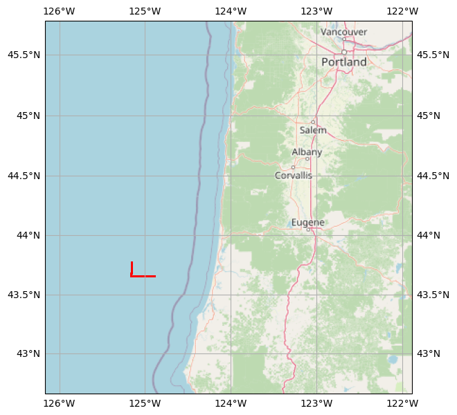
    duplicate_ping_times:         0

1.4. Extract and plot GPS locations from Platform group#

Extract and join the latitude and longitude variables from the Platform group in the combined_ed EchoData object. Convert to a Pandas DataFrame first, then to a GeoPandas GeoDataFrame for convenient viewing and manipulation.

gps_df = combined_ed['Platform'].latitude.to_dataframe().join(combined_ed['Platform'].longitude.to_dataframe())
gps_df.head(3)

	latitude	longitude
time1
2017-07-28 18:16:21.475999744	43.657532	-124.887015
2017-07-28 18:16:21.635000320	43.657500	-124.887000
2017-07-28 18:16:22.168999936	43.657532	-124.887080

gps_gdf = gpd.GeoDataFrame(
    gps_df,
    geometry=gpd.points_from_xy(gps_df['longitude'], gps_df['latitude']), 
    crs="epsg:4326"
)

Create a cartopy reference map from the point GeoDataFrame, to place the GPS track in its geographical context.

basemap = cimgt.OSM()
_, ax = plt.subplots(
    figsize=(7, 7), subplot_kw={"projection": basemap.crs}
)
bnd = gps_gdf.geometry.bounds
ax.set_extent([bnd.minx.min() - 1, bnd.maxx.max() + 3, 
               bnd.miny.min() - 1, bnd.maxy.max() + 2])
ax.add_image(basemap, 7)
ax.gridlines(draw_labels=True, xformatter=LONGITUDE_FORMATTER, yformatter=LATITUDE_FORMATTER)
gps_gdf.plot(ax=ax, markersize=0.1, color='red', 
             transform=ccrs.PlateCarree());

1.5. Compute mean volume backscattering strength (\(\text{MVBS}\)) and plot interactive echograms using `hvplot`#

echopype supports basic processing funcionalities including calibration (from raw instrument data records to volume backscattering strength, \(S_V\)), denoising, and computing mean volume backscattering strength, \(\overline{S_V}\) or \(\text{MVBS}\). The EchoData object can be passed into various calibration and preprocessing functions without having to write out any intermediate files.

We’ll calibrate the combined backscatter data to obtain \(S_V\). For EK60 data, by default the function uses environmental (sound speed and absorption) and calibration parameters stored in the data file. Users can optionally specify other parameter choices. \(S_V\) is then binned along range (depth) and ping time to generate \(\text{MVBS}\).

Sv_ds = ep.calibrate.compute_Sv(combined_ed).compute()
MVBS_ds = ep.preprocess.compute_MVBS(
    Sv_ds,
    range_meter_bin=5,  # in meters
    ping_time_bin='20s'  # in seconds
)

Replace the channel dimension and coordinate with the frequency_nominal variable containing actual frequency values. Note that this step is possible only because there are no duplicated frequencies present.

MVBS_ds = ep.consolidate.swap_dims_channel_frequency(MVBS_ds)

List the three frequencies used by the echosounder

MVBS_ds.frequency_nominal.values

array([ 18000.,  38000., 120000.])

Generate an interactive plot of the three \(\text{MVBS}\) echograms, one for each frequency. The frequency can be changed via the slider widget.

MVBS_ds["Sv"].hvplot.image(
    x='ping_time', y='echo_range', 
    color='Sv', rasterize=True, 
    cmap='jet', clim=(-80, -50),
    xlabel='Time (UTC)',
    ylabel='Depth (m)'
).options(width=500, invert_yaxis=True)

1.6. Package versions#

import datetime, s3fs
print(f"echopype: {ep.__version__}, xarray: {xr.__version__}, geopandas: {gpd.__version__}, "
      f"fsspec: {fsspec.__version__}, s3fs: {s3fs.__version__}")

print(f"\n{datetime.datetime.utcnow()} +00:00")

echopype: 0.6.3, xarray: 2022.3.0, geopandas: 0.11.1, fsspec: 2022.8.2, s3fs: 2022.8.2

2022-10-19 01:44:10.332040 +00:00

Echopype Examples

echopype Tour

Contents

1. echopype Tour#

1.1. Introduction#

1.1.1. Goals#

1.1.2. Description#

1.1.3. Running the notebook#

1.2. Compile list of raw files to read from the NCEI WCSD S3 bucket#

1.3. Read target raw files directly from AWS S3 bucket and convert to netcdf#

1.4. Extract and plot GPS locations from Platform group#

1.5. Compute mean volume backscattering strength (\(\text{MVBS}\)) and plot interactive echograms using `hvplot`#

1.6. Package versions#

Echopype Examples

echopype Tour

Contents

1. echopype Tour#

1.1. Introduction#

1.1.1. Goals#

1.1.2. Description#

1.1.3. Running the notebook#

1.2. Compile list of raw files to read from the NCEI WCSD S3 bucket#

1.3. Read target raw files directly from AWS S3 bucket and convert to netcdf#

1.4. Extract and plot GPS locations from Platform group#

1.5. Compute mean volume backscattering strength (\(\text{MVBS}\)) and plot interactive echograms using hvplot#

1.6. Package versions#

1.5. Compute mean volume backscattering strength (\(\text{MVBS}\)) and plot interactive echograms using `hvplot`#